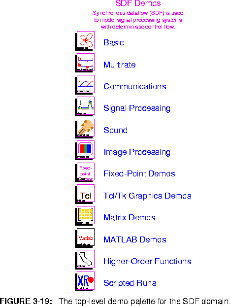


A rather large number of SDF demonstrations have been developed. These can serve as valuable illustrations of the possibilities. Almost every star is illustrated in the demos. Because of the large number, the demos are organized into a set of palettes. Certain demos may appear in more than one palette. A top-level palette, shown in figure 3-19, contains an icon for each demo palette. Notice that the demo palettes collect the hierarchy in a single column, whereas the star palettes collect the hierarchy in two columns.
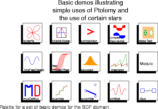
These demos illustrate the use of certain stars without necessarily performing functions that are sophisticated. The palette is shown in figure
3-20. The demos are described below from left to right, top to bottom.
butterfly
Use sines and cosines to compute a curve known as the butterfly curve, invented by T. Fay. The curve is plotted in polar form.
chaoticNoise
Chaotic Markov map example with a nonlinear feedback loop.
comparison
Compare two sinusoidal signals using the Test star.
delayTest
Illustrates the use of initializable delays.
lmsFreqDetect
Illustrate the use of the LMS algorithm to estimate the dominant sinusoidal frequency in the input signal.
freqPhaseOffset
Impose frequency jitter and phase offset on a sinusoid using the freqPhase SDF block.
gaussian
Generate a Gaussian white noise signal, and plot its histogram and estimated autocorrelation.
integrator
Demonstrate the features of the integrator star, such as limiting, leakage, and resetting.
Modulo
Demonstrate modulus computation for float and integer data types.
muxDeMux
Demonstrate the Mux and DeMux stars, which perform multiplexing and demultiplexing. Contrast with the scramble demo below.
quantize
Demonstrate the use of the Quantizer star.
scramble
This system rearranges the order of samples of signal using the Commutator and Distributor stars. Note that because these are multirate stars, one iteration involves more than one sample. Contrast with the muxDeMux demo above. 
sinMod
Modulate a sinusoid by multiplying by another sinusoid.
tbus
Illustrate the bus facility in Ptolemy, in which multiple signals are combined onto a single graphical connection.
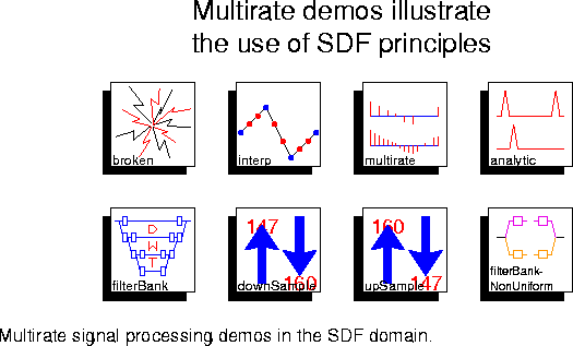
The demos with icons shown in figure
3-21
 illustrate synchronous dataflow principles as applied to multirate signal processing problems. These are arranged roughly in order of sophistication.
broken
Give an example of an inconsistent SDF system. It fails to run, generating an error message instead.
interp
Use an FIR filter to upsample by a factor of 8 and linearly interpolate between samples.
multirate
Upsample a sinusoidal signal by a ratio of 5/2 using a polyphase lowpass interpolating FIR filter.
analytic
Use a FIRCx star filter to reduce the sample rate of a sinusoid by a factor of 8/5, and at the same time produce a complex approximately analytic signal (one that has no negative frequency components).
filterBank
Implement an eight-level perfect reconstruction one-dimensional filter bank based on the biorthogonal wavelet decomposition.
downSample
Convert from the digital audio tape sampling rate (48 kHz) to the compact disc sampling rate (44.1 kHz). The conversion is performed in multiple stages for better performance.
upSample
Convert from the compact disc sampling rate (44.1 kHz) to the digital audio tape sampling rate (48 kHz). The conversion is performed in multiple stages for better performance.
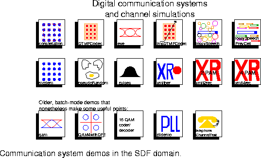
 3-22 points to some examples of digital communication systems and channel simulators. This palette has been steadily growing.
constellation
A 16-QAM signal is sent through a baseband equivalent channel that simulates the following impairments: frequency offset, phase jitter and white Gaussian noise.
DTMFCodec
Dual-Tone Modulated Frequency Demo. Generate touch tones and decode the based on the Goertzel Algorithm.
eye
Plot an eye diagram for a binary anitpodal signal with a raised-cosine pulse shape and user controlled noise.
lmsDTMFCodec
Dual-Tone Modulated Frequency Demo. Generate touch tones
and decode the based on the LMS Algorithm.
lossySpeech
Illustrate the effect on speech of a zero-substitution policy in a network (such as ATM) with 48 byte packets and a variable loss probability. Note that this demo requires audio capability and will probably only work on Sun workstations.
lossySpeechPrevCell
Illustrate the effect on speech of a previous cell substitution policy in a network (such as ATM) with 48 byte packets and a variable loss probability. Note that this demo requires audio capability and will probably only work on Sun workstations.
modem
Baseband model of a 16-QAM modem.
pseudoRandom
Generate a pseudo-random sequence of zeros and ones using a maximal-length shift register and test its randomness by estimating it autocorrelation.
pulses
Generate raised cosine and square-root raised cosine pulses and demonstrate matched filtering with the square-root raised cosine pulse.
xmitber
Bit Error determination through simulation at various noise levels.
xmit2rec
Simple 2-level PAM communication system (matched filtering at the receiver).
xmit4rec
Simple 4-level PAM communication system (no filtering at the receiver).
qam
Produce a 16-point quadrature amplitude modulated (QAM) signal and displays the eye diagram for the in-phase part, the constellation, and the modulated transmit signal.
QAM4withDFE
This is a model of a digital communication system that uses quadrature amplitude modulation (QAM) and a fractionally spaced decision feedback equalizer.
codeDecode
Encode and decode a 16-QAM signal using differential encoding for the quadrant and Gray coding for the point within the quadrant.
plldemo
Simulate a fourth-power optical phase-locked loop with laser phase noise and additive Gaussian white noise operating on a complex baseband envelope model of the signal.
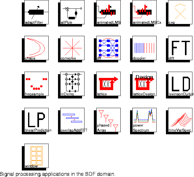
 3-23. Several of these serve as good examples to help in solving the exercises included at the end of the chapter.
adaptFilter
An LMS adaptive filter converges so that its transfer function matches that of a fixed FIR filter.
allPole
Two realizations of an all-pole filter are shown to be equivalent. One uses an FIR filter in a feedback path, the other uses the BlockAllPole star.
animatedLMS
An LMS adaptive filter is configured as in the adaptFilter demo, but this time the filter taps are displayed as they adapt.
animatedLMSCx
A complex LMS adaptive filter is configured as in the adaptFilter demo, but in addition, user-controlled noise is added to the feedback loop using an on-screen slider to control the amount of noise. The filter taps are displayed as they adapt.
cep
Given the coefficients of any polynomial, this demo uses the cepstrum to find a minimum-phase polynomial. Thus, given the coefficients of the denominator polynomial of an unstable filter, this demo will compute the coefficients of a stable denominator polynomial that has the same magnitude frequency response.
chaos
This is a simple demonstration of chaos, in which the phase-space plot of the famous Henon map is given.
convolve
Convolve two rectangular pulses in order to demonstrate the Convolve star.
dft
Compute a discrete Fourier transform of a finite signal using the FFT star. The magnitude and phase (unwrapped) are plotted.
doppler
A sine wave is subjected to four successive amounts of doppler shift. The doppler shift is accomplished by the phaseShift galaxy, which forms an analytic signal (using a Hilbert transform) that modulates a complex exponential.
dtft
Demonstrate the DTFT star, showing how it is different from the FFTCx star. Specifically, the range, number, and spacing of frequency samples is arbitrary.
freqsample
This system designs FIR filters using the frequency sampling method. Samples of the frequency response are converted into FIR filter coefficients.
iirDemo
Two equivalent impementations of IIR filtering. This demo is not present in Ptolemy0.6.
lattice
Demonstrate the use of lattice filters to synthesize an auto-regressive (AR) random process.
latticeDesign
Use of Levinson-Durbin algorithm to design a lattice filter with a specified transfer function.
levinsonDurbin
Use the Levinson-Durbin algorithm to estimate the parameters of an AR process.
linearPrediction
Perform linear prediction on a test signal consisting of three sinusoids in colored, Gaussian noise. Two mechanisms (Burg's algorithm and an LMS adaptive filter) for linear prediction are compared.
overlapAddFFT
Convolution is implemented in the frequency domain using overlap and add.
phasedArray
Simulate a plane wave approaching a phased array with four sensors. The plane wave approaches from angles starting from head on and slowly rotating 360 degrees. The response of the antenna is plotted as a function of direction of arrival in polar form.
powerSpectrum
Compare three methods for estimating a power spectrum of a signal with three sinusoids plus colored noise. The three methods are the periodogram method, the autocorrelation method, and Burg's method.
timeVarSpec
A time-varying spectrum is computed using the autocorrelation method and displayed using a waterfall plot.
window
Generate and display four window functions and the magnitude of their Fourier transforms. The windows displayed are the Hanning, Hamming, Blackman, and steep Blackman.
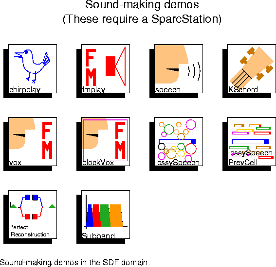
The demos in the palette in figure
3-24
 assume that a program called
 ptplay is in your path, and that it accepts data of an appropriate format and will play it over a workstation speaker at an 8 kHz sample rate. If you are using a Sun SPARCStation, these conditions will most likely be satisfied, if your path is correct. The ptplay program has also been used on SGI Indigos and HP 700s and 800s. If you are on an HP, you may need other publicly available software.The samples are written into a file before they are played. Since a large number of samples must be generated, these demos can take some time to run. By contrast, the CGC domain has some audio demos that generate sounds in real time at 8 kHz, assuming a reasonably fast workstation.
chirpplay
Chirp generator that plays on the workstation speaker.
fmplay
Sound generator using FM modulation that plays on the workstation speaker.
speech
Read a speech signal from a file, and encode it at two bits per sample using adaptive differential pulse code modulation with a feedback-around-quantizer structure. The signal is then reconstructed from the quantized data. The original and reconstructed speech are played over the workstation speaker.
KSchord
Simulation of plucked string sounds using the Karplus-Strong algorithm.
vox
Coarticulation with an Adaptive Vocoder. The resulting FM synthesized sound is played over the workstation speaker.
blockVox
A block processed version of the vox demo.
lossySpeech
Illustrate the effect on speech of a zero-substitution policy in a network (such as ATM) with 48 byte packets and a variable loss probability. This demo also appears in the basic demos palette
lossySpeechPrevCell
Illustrate the effect on speech of a previous cell substitution policy in a network (such as ATM) with 48 byte packets and a variable loss probability. This demo also appears in the basic demos palette.
perfectReconstuction
Eight-channel perfect reconstruction one-dimensional analysis/synthesis filterbank. The incoming speech signal is split into eight adjacent frequency bins and then reconstructed. The original and reconstructed speech are played over the workstation speaker.
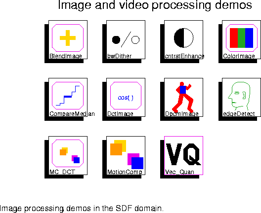
The demos in figure  3-25 all read images from files on the workstation disk, process them, and then display them. Some of the demos process short sequences of images, thus illustrating video processing in Ptolemy. They all use the image classes described in
"Image processing stars" on page 3-105. The set of demos in this palette does not reflect the richness of possibilities. See the DE domain for more image and video signal processing applications in the context of packet-switched network simulations. The video display requires that the Utah Raster Toolkit be installed and available in the user's path.
BlendImage
Combine two images and display the result.
bwDither
Demonstrate four different forms of black and white dithering: error diffusion, clustered dither, dispersed dither, and use custom mask.
cntrastEnhance
Contrast enhancement by histogram modification.
ColorImage
Convert an RGB (red-green-blue) format color image to YUV (luminance-hue-saturation) format and back, and then display it on the workstation screen.
CompareMedian
Median filter an image to reduce artifacts due to interleaved scanning in video sequences.
DctImage
Perform discrete cosine transform (DCT) coding of an image sequence.
DpcmImage
Perform differential pulse code modulation (DPCM) on an image sequence.
EdgeDetect
Demonstrate four different forms of edge detection: Sobel, Roberts, Prewitt, and Frei-Chen.
MC_DCT
Perform motion compensation and DCT encoding of video.
MotionComp
Perform motion compensation video coding.
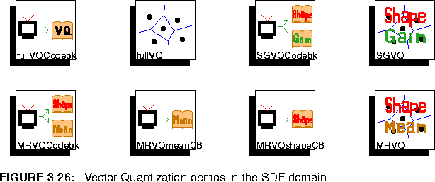
- The Vec_Quan icon in the image processing palette brings up a sub-palette that has several vector quantization demonstrations in figure
3-26
 :
:
fullVQCodebk
- Generate a codebook for full search vector quantization.
fullVQ
- Full search vector quantization using codebook generated by
fullVQCodebk.
SGVQCodebk
- Generate codebooks for shape-gain vector quantization.
SGVQ
- Shape-gain vector quantization using codebook from
SGVQCodebk.
MRVQCodeBk
- Generate codebooks for mean-removed vector quantization using independent quantizer structure.
MRVQmeanCB
- Generate codebook for mean-removed vector quantization.
MRVQshapeCB
- Generate the shape codebook for mean-removed quantization using alternate structure. This universe uses the codebook generated by
MRVQmeanCB.
MRVQ
- Mean-removed vector quantization.
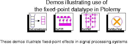
The demos shown in figure 3-27 illustrate the use of fixed-point stars in the SDF domain. These stars are used to model hardware implementations with finite precision.
fixConversion
Illustration of the different masking options available.
fixFIR
Effect of filter tap precision on the frequency response.
fixIIRdf
Comparison of a fourth-order direct-form IIR filter implemented with floating-point arithmetic and a similar filter implemented with fixed-point arithmetic.
fixMpyTest
Testing of fixed-point multiplication over a range of numbers by comparison against floating-point multiplication. The results should be the same.
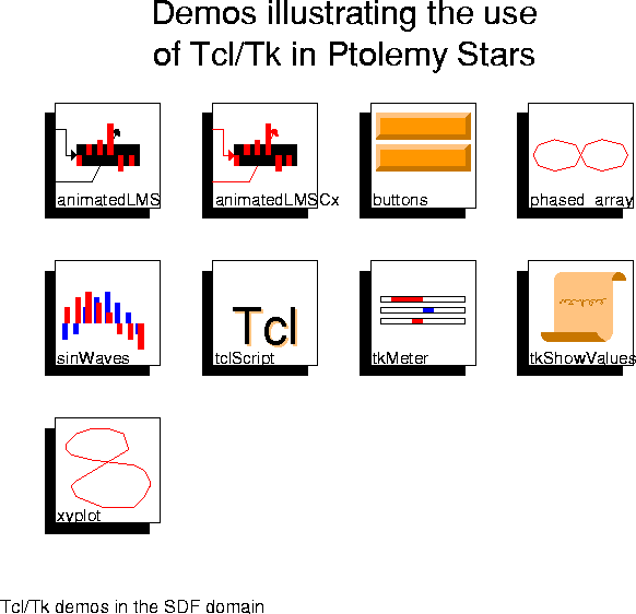
These demos shown in figure  allow the user to interact with the simulation. The interactivity is provided by the Tcl scripting language controlling the Tk graphics toolkit. Tcl is integrated throughout Ptolemy. Tk has been integrated into the graphical user interfaces for Ptolemy, but not in the ptcl textual interpreter. Therefore, these stars do not work in ptcl.
animatedLMS
animatedLMSCx
buttons
Demonstrate TkButtons.
phased_Array
Demonstrate TkSlider by creating a vertical array of radar sensors that can be move in the horizontal plane. Note that small movements of the sensors radically change the polar gain plot. This simulation demonstrates the importance of sensor calibration to performance of the sensor array.
sinWaves
Demonstrate TkBarGraph by generating and displaying a complex exponential.
tclScript
Demonstrate TclScript by generating two interactive X window follies that consist of circles that move in the same playing field.
tkMeter
Demonstrate TkMeter by creating three bar meters. The first oscillates sinusoidally. The second displays a random number between zero and one. The third displays a random walk.
tkShowValues
Demonstrate TkShowValues and TkText by displaying the ASCII form of two ramp sequences.
xyplot
Demonstrate the dynamic plotting capabilities of the xyplot star.
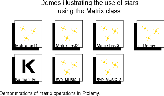
The systems in figure 3-29 demonstrate the use of matrix particles in Ptolemy. Matrices are also used in the SDF domain to represent images.
See "Image and video processing demos" on page 3-120. The demonstrations below are primarily to test matrix operations.
MatrixTest1
Demonstrate the use of the Matrix stars that have one input. These include the operations inverse, transpose, and multiply by a scalar gain for all matrix types. Also conjugate and Hermitian transpose are available for the complex matrix type.
MatrixTest2
Demonstrate the use of some simple Matrix stars with two inputs. These include multiply, add, and subtract.
MatrixTest3
Demonstrate the use of the Matrix conversion stars. These convert between the scalar particles and the matrix particles as well as between the various matrix types.
initDelays
Illustrate the use of initializable delays with the matrix class.
Kalman_M
Compare the convergence properties of a Kalman filter to those of an LMS filter when addressing the problem of adaptive equalization of a process in noise.
SVD_MUSIC_1
Show the use of singular-value decomposition (SVD) and the Multiple-Signal Characterization (MUSIC) algorithm to identify the frequency of a single sinusoid in a signal that has two different signal to noise ratios.
SVD_MUSIC_2
Demonstrate the use of the Multiple-Signal Characterization (MUSIC) algorithm to identify three sinusoids in noise that have frequencies very close to each other.
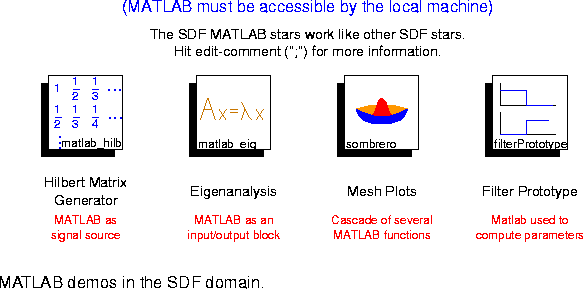
The demos pictured in figure
3-30 illustrate the use of the MATLAB stars. The MATLAB stars convert input values into MATLAB matrices, apply a sequence of MATLAB commands to the matrices, and output the result as Ptolemy matrices. The filterPrototype demonstration shows how to use MATLAB to compute parameters of stars.
matlab_hilb
This demo uses MATLAB as a signal source to produce a Hilbert matrix. The Hilbert matrix is an ill-conditioned matrix used to test the robustness of numerical linear algebra routines. The matrix element (i,j) has the value of 1 / (i + j - 1). The matrix values appear similar to the coefficients of a discrete Hilbert transformer.
matlab_eig
This demo shows the use of MATLAB to perform eigendecomposition of a 2 x 2 Hermitian symmetrix complex matrix. A matrix of eigenvectors and a matrix of eigenvalues are produced. The eigenvalues are real because the input matrix is Hermitian symmetric
sombrero
This demo is an entire universe composed of a cascade of four MATLAB stars. The MATLAB stars are used a signal source and a signal sink. The overall system generates and plots a mathematical model of a two-dimensional sinc function that resembles a sombrero.
filterPrototype
This system uses a halfband lowpass filter prototype for the lowpass and highpass filters. All parameters are computed using MATLAB.
The Higher Order Function demos are described in the HOF domain chapter.
See "An overview of HOF demos" on page 4-164.
A scripted run executes the tcl code in the run control panel tcl script window. Scripted runs can be used to set up interactive tutorials.The demos shown in figure
3-31
 illustrate the use of scripted runs.
demoscript
An interactive tutorial that leads a user through a session that runs a simple universe.
sinescript
This demo runs the same sine wave modulation universe three times, each time with a different frequency.
xmitber
This demo runs a bit error determination universe at various noise levels and then plots the output.


Copyright © 1990-1997, University of California. All rights
reserved.
